From "Why Geometry Does Not Compress Weights" — to the architecture that creates this asymmetry.
Date: 2026-09-16 · Author: Millog · License: CC BY-SA 4.0
Data and code: cmq_experiment/tied_vs_untied/ (experiments H1–H4, Exp5–7), cmq_experiment/results_v6/ (quantization study)
Abstract
We test the hypothesis that weight tying — an architectural constraint standard in small LLMs — acts as an implicit regularizer: gradient interference on the shared input/output matrix deforms the embedding space into an anisotropic cone, and the network compensates by building a low-dimensional attractor ("dynamic hourglass") somewhere deep in the stack. We measured this directly on six local base models ranging from 0.135B to 5.12B parameters, including a tied-vs-untied control pair (Qwen2.5-0.5B and TinyLlama-1.1B) where the constraint is removed in one of the two models.
Results: (1) no gradient opposition exists — the paths are orthogonal everywhere (|cos| ≤ 0.023); interference manifests as dominance of one path ("tyranny of the output" in 4 out of 6 models, inversion to the input path in Gemma). (2) The hourglass is confirmed on 5 out of 6 models; the compressed zone covers up to 62% of stack depth — the "neck" is not a single layer but a wide band. (3) The spectral asymmetry "law vs trajectory" is confirmed: full-rank dense weights against low-dimensional activations — this is the mechanism behind the failure of geometric weight compression in our previous study. (4) Cross-model analysis shows generational drift of the shape of low-dimensional zones: from an early bottleneck at the input (Qwen2.5, TinyLlama), through centered hourglasses (SmolLM), to blending of compressed layers in the waist (Qwen3-4B — three minima L7/L11/L17) and further into a distributed regime without mid-stack compression (Gemma-4, sliding-window attention). (5) The "pressure of mass" hypothesis is locally falsified up to 8192 tokens: neither quality degradation nor lost-in-the-middle reproduces — geometry is flat with respect to context length.
Introduction
Computational Meat and the Illusion of Understanding
Language is "computational meat." To understand its architecture, one has to stop asking "what does the model do?" and start asking "how does it compute that?". We cannot look inside a neural network as we would into program code, but we can measure its internal states.
This article continues my previous study "Why Geometry Does Not Compress Weights" (see cmq_experiment/results_v6/). There I showed that LLM activations lie in a narrow cone: 90% of the energy is in ~1–3 principal components, while the weights are full-rank and dense. All geometric weight-compression techniques (Hadamard rotation, Lloyd-Max, conic decomposition, QJL) yielded zero or negative; the only working lever — data-adaptive error compensation (GPTQ). The final formula: weights = law of dynamics, activations = trajectory on a low-dimensional attractor.
But the main question remained: what creates this asymmetry? Why does training lead to dense weights and narrow representations? I proposed an architectural-origin hypothesis: tying the input and output matrices is an implicit regularizer that deforms the embedding space into a cone. And if this cone exists, then somewhere deep in the network must "compress" information down to low dimensionality, and at the output "expand" it back out. That is what dynamic hourglass means: not a static structure of weights but a pattern that emerges when data passes through the model.
In this article we test four hypotheses from which this picture follows:
- H1 — Gradient interference. If the input and output matrices are one and the same, then gradients from the input path (embedding) and the output path (lm_head) interfere on the shared matrix. This creates an optimization conflict: the input path pulls embeddings in one direction, the output path in another. The result is anisotropic deformation of the embedding space.
- H2 — Hourglass. If the space is compressed at the input (cone), then somewhere in the middle of the network must occur "expansion" to full dimensionality so that the model can process information, and afterwards a "compression" back for output. This creates an effective-dimensionality profile across layers: narrow → wide → narrow.
- H3 — Spectral asymmetry. Weights should be full-rank (high effective dimensionality) and activations low-dimensional (low effective dimensionality). This is a direct consequence of H1 and H2: weights are encoded as "law" (dense, cleaned by training), while representations — as "trajectory on an attractor".
- H4 — Pressure of mass. If the model uses low-dimensional representations to save compute, then as context grows it should degrade more strongly than a model with full-rank representations. This is the "lost in the middle" prediction as a geometric effect: a low-dimensional space cannot hold information from all positions of a long context.
Experimental design: for each hypothesis there is a direct measurement (tied-vs-untied control pair) and a cross-model extension (6 models from 0.135B to 5.12B). Result: two hypotheses were confirmed (H2 — on five out of six models, H3), one was confirmed in an anomalous form (H1: not gradient opposition but tyranny of one path), and the fourth is locally falsified (H4). The cross-model extension yielded a new result — a quantitatively describable drift of hourglass shape across architectural generations: from early bottleneck to centered hourglasses with blending of compressed layers, and further.
Starting Point: Why Geometry Does Not Compress Weights
So that this article reads as a continuation, let me fix what is already known from the previous study (CHMC v1→v6, results_v6/).
We tried to apply the conic geometry of activations to compression of the weights themselves: weighted SVD along the cone, adaptive ranks, covariance corrections. The path ran from collapse (ratio 4894× in v1) to parity (~1.18× in v6 at equal bit budget BPW = 4.2875 — exactly GPTQ's budget). Result on three models: SmolLM — parity with GPTQ (mean 1.179–1.186 against 1.176), Qwen2.5-0.5B — loss (single run, 1.174 against 1.141), TinyLlama-1.1B — a real win of more than 30σ (1.059 against 1.081).
All geometric techniques on weights failed: Hadamard rotation — ratio 2.23×, Lloyd-Max — 1.35× at baseline 1.21×, Cone-Aware — 2.15×, QJL — PPL 267/228 (theoretical error bound √(1−1/4) ≈ 87%). The only working lever — dampening of the Hessian estimate (λ=0.05, −4%), i.e., noise control rather than capturing geometry. Across the ensemble of 124 experiments the only flag with a positive correlation to success — dampening (+0.40); all geometric flags are around zero or negative. Low-rank drift correction was falsified against a pre-declared criterion: d90 of drift = 227–792 instead of expected <50.
The key spectral facts that this article explains architecturally: activations — a narrow cone (d90 ≈ 9 out of 576 dimensions in SmolLM, mean cosine ≈ 0.75; in middle blocks up to 98.9% of variance lies in three principal components against 13–43% at the edges), weights — dense (minimal effective rank 29–30, median ~60). The question we pose here: where does this asymmetry come from? If it were a property of data or function, geometric weight compression should work. It does not — so the source lies in model architecture, and the main candidate at architectural level is weight tying.
Part 1. Philosophy of the Hourglass
Working Metaphor
Imagine a transformer as a dynamic system: input embedding → L transformer blocks → output lm_head. If we represent the "dimensionality" of data at each step, we expect a pattern: narrow (embeddings in a cone) → wide (information is processed in full dimensionality) → narrow (output back into the cone). This is the hourglass.
Important: this is not a static structure of weights but a pattern of representations as data passes through. The weights may be full-rank everywhere, while representations are low-dimensional at the edges and high-dimensional in the middle. The hourglass is a property of the function, not of the parameters.
Why This Is Better Than "Superposition"
The mechanistic-interpretability literature has the concept of "superposition": a model packs more concepts than dimensions by overlapping directions. That explains why weights are dense and full-rank. But superposition is a static model: it says what is encoded in the weight matrices.
The hourglass is a dynamic model: it tells how data flows through the network. It explains not only the density of the weights (the law must be complete to hold the trajectory) but also the low dimensionality of activations (the trajectory lies on an attractor), and the linear accumulation of error under quantization (perturbed dynamics deflects the trajectory, but the attractor pulls it back — divergence is linear, not exponential). One dynamic picture explains all three observations; static superposition — only the first.
The Memory Paradox
If representations are compressed to low dimensionality, how does a model remember long context? The KV cache stores keys and values in full (or nearly full) dimensionality — memory is not compressed as aggressively as computational states. This predicts: as context grows, pressure on low-dimensional representations should grow, because information from all positions must "pass through" the narrow waist of the hourglass. If the model copes — then either the waist is wide enough or memory bypasses it. We will check this in H4.
Part 2. Data and Protocols
Models
Six local base models from three families (Llama/Qwen/Gemma), all measured on physical GPU 1 (cuda:1 hardcoded in the scripts); fp32 where memory allows (VRAM 15.93 GiB), otherwise bf16. Gemma uses an isolated environment .venv-gemma4 (transformers 5.17.0), since its architecture is incompatible with the transformers of the other models; the vision module was excluded from all measurements.
| Model | Architecture | Parameters (exact) | hidden | Layers | Tying? | Vocab | max_pos |
|---|---|---|---|---|---|---|---|
| smollm-135m | LlamaForCausalLM | 134,515,008 | 576 | 30 | yes | 49,152 | 2,048 |
| qwen2.5-0.5b | Qwen2ForCausalLM | 494,032,768 | 896 | 24 | yes | 151,936 | 32,768 |
| tinyllama-1.1b | LlamaForCausalLM | 1,100,048,384 | 2048 | 22 | no | 32,000 | 2,048 |
| qwen2.5-3b | Qwen2ForCausalLM | 3,085,938,688 | 2048 | 36 | yes | 151,936 | 32,768 |
| qwen3-4b | Qwen3ForCausalLM | 4,022,468,096 | 2560 | 36 | yes | 151,936 | 40,960 |
| gemma-4-e2b | Gemma4ForConditionalGeneration | 5,123,178,979 | 1536 | 35 | yes | 262,144 | 131,072 |
Control pair: Qwen2.5-0.5B (tied) and TinyLlama-1.1B (untied) — the only model in the sample without weight tying; its input matrix (wte) and output matrix (lm_head) are separate, which allows measuring H1 "before" and "after" the regularizer.
Corpus: 4 markdown documents of the cmq_experiment project (README.md, PROJECT.md, FINAL_REPORT_v4.md, report.md). Token pool: up to 8599 (Qwen tokenizer) / ~10080–10082 (Llama family); the difference in pool size — different BPE vocabularies cut the same text into a different number of pieces. The whole corpus fits into the context of models with max_pos ≥ 32k; SmolLM and TinyLlama (max_pos = 2048) used a corpus window — hence their length L=2048 in Exp6.
Measurement Protocols
- Exp7/H1. 128 tokens. G_total — backward of the built-in CE-loss. G_in — frozen clone of lm_head, backward of CE over the input path (only embeddings updated). G_out — no_grad hidden states + a fresh copy W', manual CE with HF shift (only output matrix updated). For untied models both gradients are taken in one backward. Proxy: per 128 tokens, cosine between the qkv0 perturbation from the embedding update and the perturbation from the weight update is computed — direct measure of conflict on shared weights.
- Exp5/H2. For each layer (levels 0..L, where level 0 = embeddings) a context of 2048 tokens is taken, hidden states are centered, exact SVD; PR = number of principal components for 90% variance. Neck = argminimum of the centered profile (PRc). Anisotropy — mean cosine between pairs of vectors of the layer (raw and centered).
- Exp3/H3. Exact SVD of gate_proj weights at the neck and incoming activations; k95(weights) against k95(activations), energy of top-10/top-3 singular directions.
- E4b (H4, geometry).
E_DC = N·‖x̄‖²/Σ‖vᵢ‖²— share of DC-energy (common direction) in last-layer states; two conditions:prefix(coherent corpus) vsmixed(shuffled blocks of 256 tokens), N ∈ {100, 1000, 4096, 8192}, one model A. - E4e/E4f (H4, function). Pattern-completion probe on model A: a unique code (
KZVX-9281+ 2 analogs) is embedded into the context at position p; lift = Δlogit(target token vs alternative) minus the control run without the needle. E4e — by length (L ∈ {100, 500, 1000, 2048, 4096, 8192}); E4f — by position: L ∈ {2048, 4096, 8192} × p = 0.05…0.95 (step 0.1) × 3 reps → 90 cells + 9 controls. - Exp6 (cross-model). Per-position lift on all six models, positions [0.05, 0.25, 0.45, 0.75, 0.95], 2 reps/cell; Inversion Contrast = Mean Lift(mid) − Mean Lift(edges); > 0 → inverted-U, < 0 → classic U / LiM direction.
All results in _work/exp{5,6,7}_metrics.json, cross_model_results.json and _work/neck_zone_stats.json; summary tables — in SUMMARY.md.
Part 3. Results
Hypothesis 1 — Gradient Interference as Tyranny of the Output
#### Method
For each model we take one run on 128 tokens. G_total is computed by backward of the built-in CE-loss (all parameters are updated). Then two "separate" gradients: G_in — with a frozen clone of lm_head, so that only the input embeddings are updated; G_out — with no_grad hidden states and a fresh copy W', manual CE with the standard HF shift, so that only the output matrix is updated. The cosine between G_in and G_out measures opposition: if the paths conflict on the shared matrix, the cosine must be substantially negative. Proxy measure: for each of the 128 tokens we compute the perturbation of the first qkv0 state from the embedding update (G_in) and from the lm_head weight update (G_out), and take the mean cosine distance — a direct measure of how different directions in representation space pull on shared weights.
#### Control Pair (original Exp1)
| Metric | Tied Qwen-0.5B (A) | Untied TinyLlama-1.1b (B) |
|---|---|---|
| cos(G_in, G_out) on the shared W | +0.018 (orthogonal) | n/a (separate matrices: cos(G_emb, G_lm) = +0.0013) |
| Norm ratio out/in (lm/emb) | 3.754 | 0.998 |
| cos(G_total, G_out) | 0.967 — output path absorbs the full update | — |
| Proxy: effect of emb-update on qkv_L0 | +0.007 | +0.002 |
In the tied model the output path dominates by norm 3.754×, and G_total nearly coincides with it (cos = 0.967): the gradient of the input role is "suppressed." In the untied model norms are balanced (ratio 0.998) and paths orthogonal (cos +0.0013): separate matrices do not interfere either. The proxy conflict in both cases is negligibly small (≤ 0.007): shared weights are not "torn" into different directions.
!
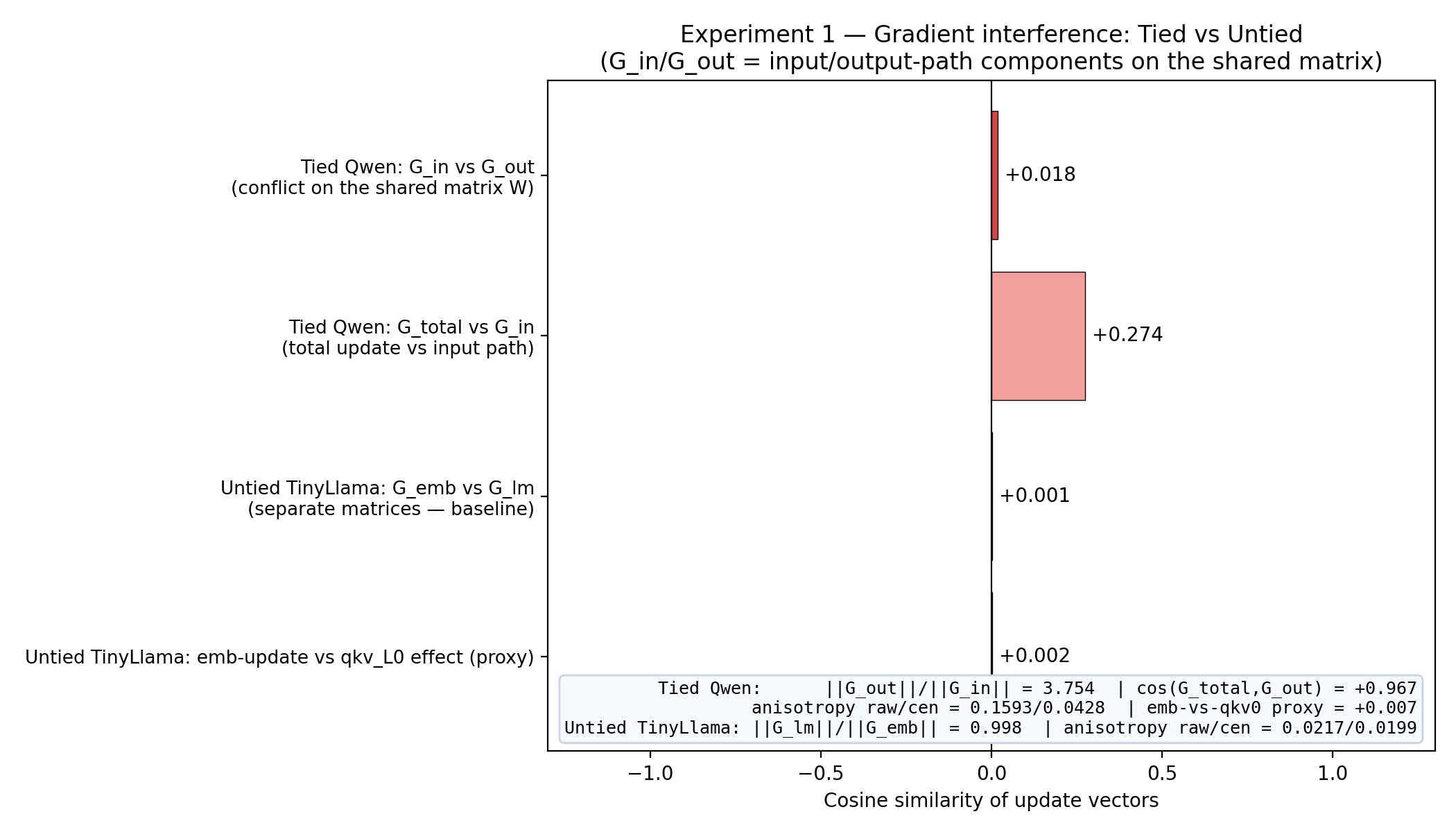
Figure 1. Gradient norms and cosines of G_in/G_out on the shared matrix: Qwen2.5-0.5B (tied, output dominates ×3.754) and TinyLlama-1.1b (untied, balanced, orthogonal).
#### Cross-model Exp7: six models
| Model | Tying? | cos(G_in,G_out) / cos(G_emb,G_lm) | ‖G_out‖/‖G_in‖ | Dominant path | Proxy emb→qkv0 |
|---|---|---|---|---|---|
| smollm-135m | yes | +0.0155 | 4.416 | output (cos(G_total,G_out) ≥ 0.967) | +0.0014 |
| qwen2.5-0.5b | yes | +0.0183 (original exp1: +0.018) | 3.754 (original: 3.754) | output | +0.0073 (original: +0.007) |
| tinyllama-1.1b (untied) | no | +0.0013 (cos G_emb,G_lm) | 0.998 (balanced) | — | +0.0022 |
| qwen2.5-3b | yes | −0.0061 | 6.953 | output | +0.1748 |
| qwen3-4b | yes | −0.0036 | 5.496 | output | +0.2231 |
| gemma-4-e2b | yes | +0.0229 | 0.021 — inversion (input dominates) | input: ‖G_in‖ = 664 vs ‖G_out‖ = 13.97, cos(G_total,G_in) = 0.9997 | +0.1197 |
Three observations.
First: there is no opposition anywhere. The G_in/G_out cosines lie in the range [−0.006, +0.023] — this is orthogonality within noise. The hypothesis "the input path pulls embeddings against output" is falsified in all six cases: the gradients of the two paths do not conflict; they are nearly perpendicular. Interference on the shared matrix is not a struggle but coexistence.
Second: interference manifests as dominance. In four out of five tied models, the output path dominates by norm ×3.75–6.95 and G_total is nearly identical to it (cos(G_total,G_out) ≥ 0.967). We call this "the tyranny of the output": the shared regularizer does not create a conflict — it makes one of the two paths negligible for the shared matrix. This same direction yields a prediction confirmed by H2: if the output path dictates the shared matrix, then embedding space is optimized for decoding (output) rather than encoding — hence its conicity.
Third: in Gemma-4 the picture is inverted. ‖G_in‖ = 664 against ‖G_out‖ = 13.97, cos(G_total,G_in) = 0.9997 — the input path dominates. Two honest caveats. First, a matrix's gradient norm depends on its size (in Gemma the embedding is 1536×262144 — the largest in the sample), so cross-model norm ratios are not compared directly; only the direction of dominance within a model is comparable. Second, in Gemma4 the output of the embedding passes through scaling (wrapper class Gemma4TextScaledWordEmbedding): the input-path gradient is differentiated through this multiplier, and at large scale ‖G_in‖ grows proportionally to it. This is the natural explanation for the inversion: not "input drowns out output" but that embedding scaling amplifies the input gradient — an interpretation verifiable by reading the scale factor from the model code. To our knowledge, this is the first documented observation of dominance inversion on a shared matrix: in the tied-decoder literature "tyranny of the output" is discussed, its inversion is not reported in any source — the regime requires separate study.
Proxy trend. The proxy conflict grows with model size: 0.0014 (SmolLM) → 0.0073 (Qwen0.5B) → 0.2231 (Qwen3-4B), and in untied TinyLlama it is minimal among the large models (0.0022). The direction matches expectation: the larger the model, the more the input and output paths "diverge" in representation space — but even the maximum of 0.22 is far from conflict; this is a moderate divergence of directions, not opposition.
!
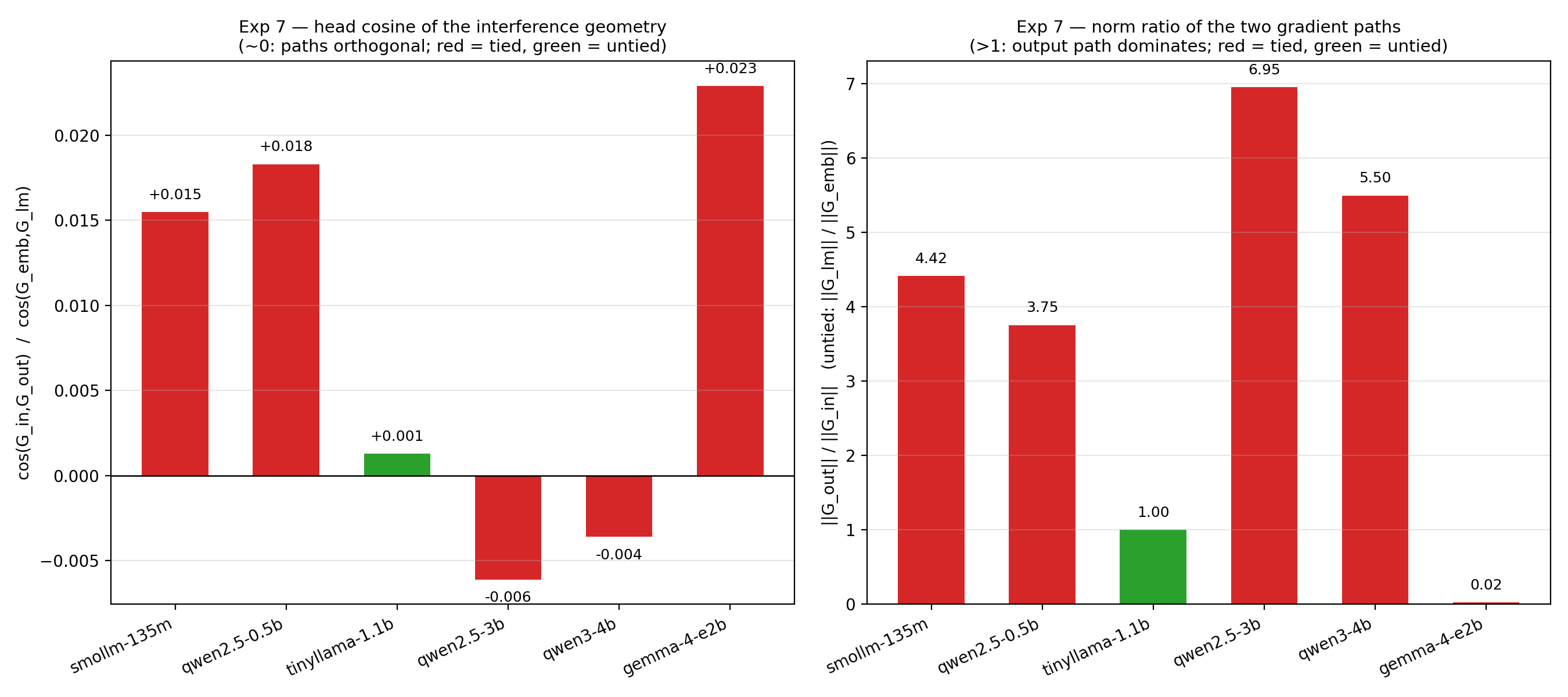
Figure 2. Input/output gradient norms and cosines across six models (Exp7): output dominance in four tied models, inversion at Gemma-4.
!
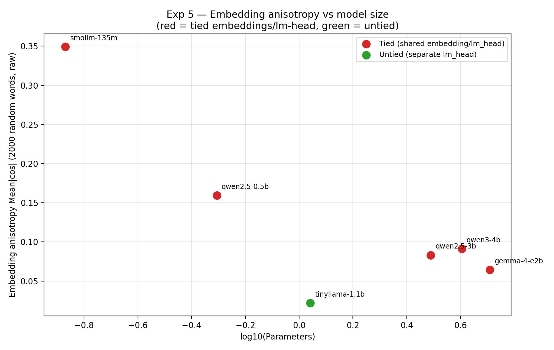
Figure 3. Anisotropy of the embedding space (raw and centered) versus size: tied models are deformed into a cone, the single untied TinyLlama — minimal anisotropy.
#### Verdict H1:PARTIALLY CONFIRMED IN ANOMALOUS FORM — reproduces on all six models
Weight tying does work as a regularizer, but the mechanism is not "gradient opposition" but dominance of one path: the shared output path sets the embedding matrix (cos(G_total,G_out) ≥ 0.967 in 4 out of 5 tied models), the input path is marginal. The proxy conflict is small everywhere, but grows monotonically with model size and is minimal in untied TinyLlama — the direction matches the hypothesis. In Gemma-4 dominance is inverted to the input path (embedding scaling), which does not break but refines the picture: the regularizer always picks one winner, but the winner depends on the architecture.
Hypothesis 2 — Universal Hourglass and Its Generational Drift
#### Method
For each stack level (0 = embeddings, 1..L = transformer blocks) we take a 2048-token context, center the hidden states by their mean, and run an exact SVD. PR — number of principal components explaining 90% of variance (raw); PRc — the same for centered states. The hourglass neck = level with minimal PRc. We additionally compute layer anisotropy — mean cosine between vector pairs (raw and centered).
#### Control Pair (original Exp2)
| Metric | Tied Qwen-0.5B (A) | Untied TinyLlama-1.1b (B) |
|---|---|---|
| PR(L0) — embeddings | 25.88 | 155.83 |
| PR mid-level (L12 / L11) | 1.37 | 2.12 |
| PR last layer | 7.64 | 30.36 |
| Neck (min centered PR) | L4, PR = 1.17 | L3, PR = 1.13 |
Both models give wide–narrow–wide: a broad input end, a narrow neck (PR ≈ 1.2 — practically rank 1), and a broader output end. The TZ criterion — "shape resembles an hourglass" (symmetry not required) — both models pass. Recorded asymmetry (caveat): collapse at the input edge (L3–L4), then a long low plateau, recovery only in the last ~5 layers — Qwen: raw PR peaks ≈91 @ L1, ≈68 @ L22–23; TinyLlama: monotonic growth to 57 @ L21. The neck is nearly identical for tied and untied (1.17 vs 1.13) → the low-dimensional attractor is a property of small LLMs on this context, not specific to tying. This is already a hint that the hourglass shape depends on the architecture, not only on weight tying.
!
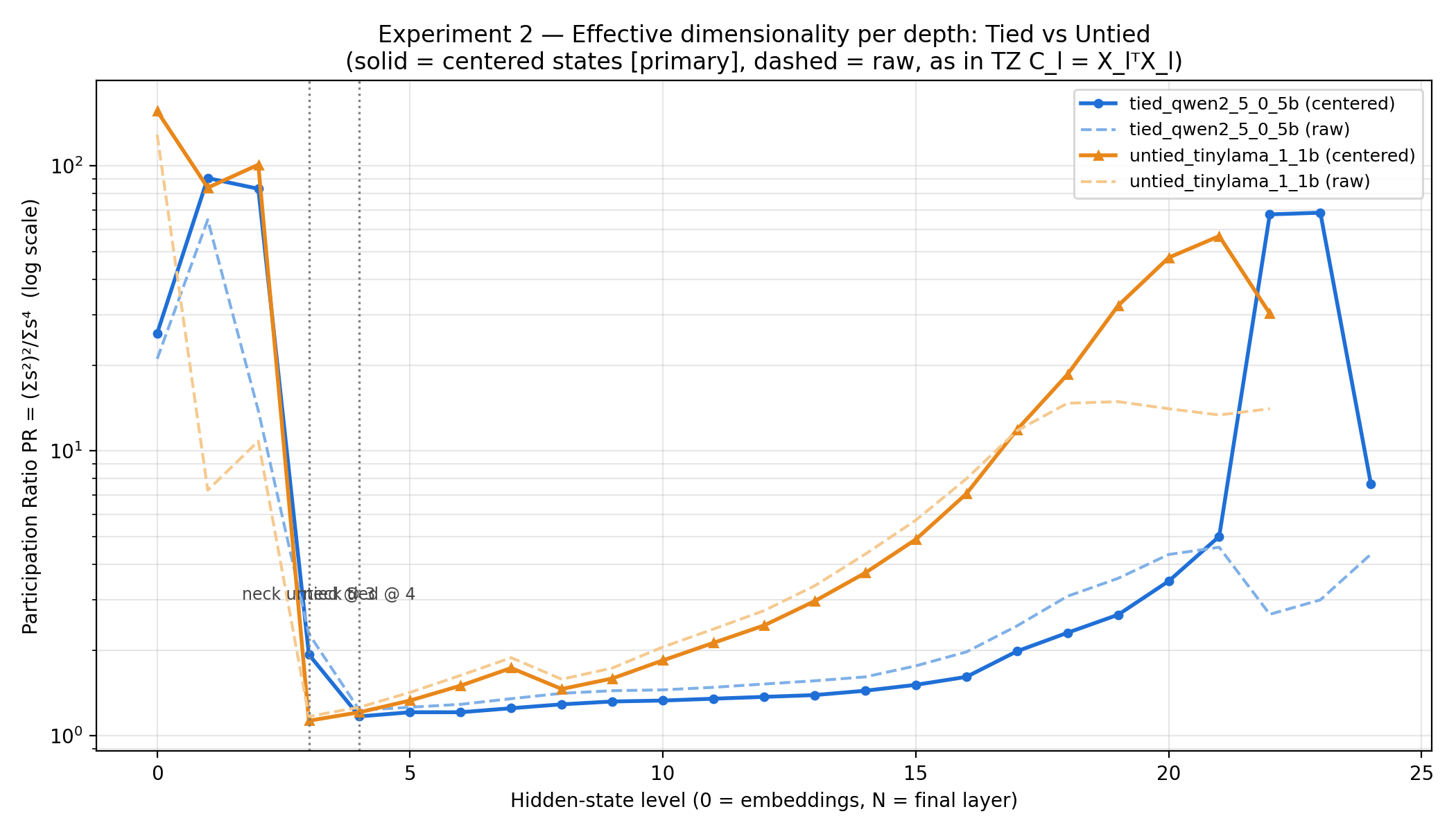
Figure 4. Principal-rank profiles across the Qwen2.5-0.5B (tied) and TinyLlama-1.1b (untied) stacks: wide–narrow–wide, neck L4 (PR 1.17) / L3 (PR 1.13), asymmetry — collapse at the input edge and recovery in the final layers.
#### Necks in Six Models (Exp5)
| Model | L | Neck (level) | Neck depth | PRc(neck) |
|---|---|---|---|---|
| smollm-135m | 30 | L12 | 40% | 1.08 |
| qwen2.5-0.5b | 24 | L4 | 17% | 1.17 |
| tinyllama-1.1b | 22 | L3 | 14% | 1.13 |
| qwen2.5-3b | 36 | L3 | 8% | 1.10 |
| qwen3-4b | 36 | L17 (middle of the stack) | 47% | 1.13 |
| gemma-4-e2b | 35 | L35 (last block before lm_head) | no mid-stack | 6.00 |
For Gemma, centered PR stays high across all layers (≈ 33–122) and drops to 6.0 only at the last level: there is no mid-stack collapse; its "bottleneck" sits at the output edge and is ~5× looser than the necks of the other models (PR 6 vs ≈ 1.1).
Embedding anisotropy (raw / centered): smollm 0.349/0.059; qwen0.5b 0.159/0.043; tinyllama 0.022/0.020; qwen3b 0.083/0.021; qwen4b 0.091/0.019; gemma 0.064/0.027. The only untied model has the minimal anisotropy (0.022) — the direction matches H1: without a shared regularizer, the embedding space is not deformed into a cone as strongly as in tied models (on the unbalanced sample 5 tied / 1 untied this is an observation, not statistics).
#### Compression Zones: From Bottleneck to Layer Mixing
The "neck" as a single minimum point — a coarse model. We characterized the low-dimensional zone quantitatively (cross_model/compute_zone_stats.py, _work/neck_zone_stats.json): n_low = number of stack levels 1..L with PRc < T=2 (PR ≈ 2 means effective rank close to 2); zone = largest connected run of sub-T levels containing the neck; local minima — internal dips of the profile below threshold.
| Model | n_low / L | Zone around neck | Width | Zone start (fraction of depth) | Local minima <2 | Regime |
|---|---|---|---|---|---|---|
| smollm-135m | 14/30 (47%) | L12–L25 | 14 (47% of depth) | 0.40 | {L12} | centered hourglass |
| qwen2.5-0.5b | 15/24 (62%) | L3–L17 | 15 (62%) | 0.12 | {L4} | early funnel |
| tinyllama-1.1b | 8/22 (36%) | L3–L10 | 8 (36%) | 0.14 | {L3, L8} | early funnel, double waist |
| qwen2.5-3b | 22/36 (61%) | L3–L24 | 22 (61%) | 0.08 | {L3} | early funnel / long shelf |
| qwen3-4b | 20/36 (56%) | L7–L26 | 20 (56%) | 0.19 | {L7, L11, L17} | centered hourglass, triple waist |
| gemma-4-e2b | 0/35 (0%) | none (<2); at T=10: only L35 (PRc 6.0) | — | 1.00 | {} | distributed regime, output compression |
Three regimes and generational drift. Old generation (Qwen2.5 ×2, TinyLlama) builds the low-dimensional zone right at the input: onset at 8–14% of depth, asymmetric funnel — a "bottleneck" in the classical sense. In TinyLlama there are two dips inside the zone (L3 and L8) — a primitive vestigial form of layer mixing. Middle generation (SmolLM) centers its zone: onset 0.40, width 14 layers, single minimum at mid-stack (L12). The new generation splits into two vectors. Qwen3-4B — the most centered hourglass in the sample (width 56% of depth), but its waist consists of three compressed minima L7/L11/L17: that is exactly "mixing of compressed layers" — the model does not fold information into a single neck, it maintains low-dimensionality as a wide band with structure inside, i.e. several attractor "nodes" distributed across the stack. Gemma-4 goes further than the hourglass: there is no mid-stack compression at all (n_low = 0 under the strict threshold; PRc across the stack 33–122), and only the final block compresses (PRc 6.0, five times looser than the necks of the other models). The likely mechanism — sliding-window attention: 28 of 35 layers operate with a window of 512 tokens, and the representation does not need global compression across the stack because each layer is local; only the output concentrates. This is an interpretation, it requires a separate experiment (window ablation), but quantitatively the picture "hourglass → distributed regime" is recorded: zone onset shifts from 0.08 to 1.00 as architectures get newer. This drift predicts differences in positional recall profiles across models — the connection is checked by the cross-model LiM scan (Exp6) given below.
Honest limitations: n = 6 models of three families, cross-comparisons are confounded by size and architecture; SmolLM — a small model with a centered zone, so "newer = more centered" is not strictly monotonic in size but describes the generational trend (Qwen2.5 → Qwen3, Gemma). Nevertheless, the shape of the zones reproduces on each model independently of size: for all five standard models the zone spans 36–62% of stack depth — "the hourglass" is not a point but an extended structure.
!
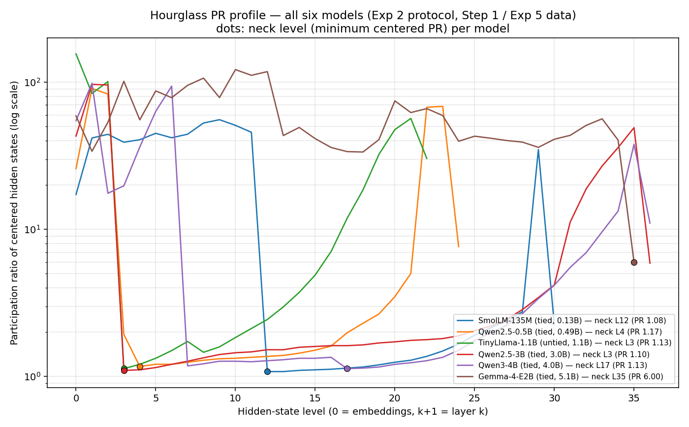
Figure 5. Full PR profiles of six models on one axis: Qwen2.5/TinyLlama funnels at the input, centered bands of SmolLM and Qwen3-4B (triple waist), flat Gemma profile with compression only at the output.
#### Verdict H2:CONFIRMED ON 5 OF 6 MODELS (Gemma — exception)
All five standard models show a low-dimensional zone in the stack with neck PRc ≈ 1.1–1.2; the zones cover up to 62% of depth, and the shape of the zones drifts across generations: early bottleneck (Qwen2.5, TinyLlama) → centered hourglass (SmolLM) → hourglass with mixing of compressed layers in the waist (Qwen3-4B: three minima L7/L11/L17) → distributed regime without a mid-stack neck (Gemma-4, probably — consequence of sliding-window attention). The universality of "one neck at the middle" is refuted; what is universal is the existence of an extended low-dimensional zone and its shift toward the output / distribution in newer architectures.
Hypothesis 3 — Spectral Asymmetry: Law vs Trajectory
#### Method
At the neck of the hourglass (L4 in Qwen, L3 in TinyLlama), we run exact SVD on the gate_proj weight matrix and its incoming activations. k95(X) = number of singular components explaining 95% of energy; top-10/top-3 energy — share of energy in the first directions.
#### Control Pair (original Exp3)
| Model | Matrix | Dimensionality | k95(weights) | k95(activations) | Top-3 activation energy | Top-10 weight energy |
|---|---|---|---|---|---|---|
| Qwen2.5-0.5B (tied) | gate_proj | 896×896 | 766/896 | 21/896 | 0.930 | 0.048 |
| TinyLlama-1.1b (untied) | gate_proj | 2048×2048 | 1610/2048 | 8/2048 | 0.944 | 0.056 |
The pattern is identical in both models, tied or not: weights are nearly full-rank (k95 ≈ 85–79% of dimensionality), activations radically low-dimensional (k95 = 21/896 ≈ 2.3%, 8/2048 ≈ 0.4%), while the top-3 directions carry 93–94% of energy and the top-10 weights — only 5%. Weight tying is not required to create this asymmetry: it reproduces in the untied model as well.